")
")
LK-29 is a smart weather station supplemented with measurement of ambient radioactivity, featuring a web interface and support for storing measured values in a database. It runs on an ESP32-S3 microcontroller with firmware written in MicroPython. The system is designed for continuous operation with minimal power consumption and remote configuration capability.

Hardvéru description

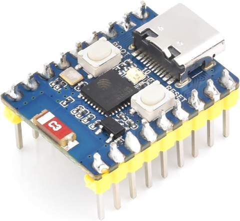 The core of the circuit solution is the ESP32-S3-Zero microcontroller; I used the Waveshare module ESP32-S3FH4R2, Type‑C USB, which integrates on the chip a dual‑core Xtensa® 32‑bit LX7 processor running at up to 240 MHz, support for 2.4 GHz Wi‑Fi (802.11 b/g/n) and Bluetooth® 5 (LE). It has built‑in 512 KB SRAM and 384 KB ROM, 4 MB Flash memory and 2 MB PSRAM. The module has a ceramic Wi‑Fi antenna soldered directly on the board, an integrated USB serial port with a full‑speed controller, 24 × GPIO pins allowing flexible configuration of individual pin functions such as 4 × SPI, 2 × I2C, 3 × UART, 2 × I2S, 2 × ADC, etc.
The overall connection diagram of the weather station is shown in the figure. The hardware core of the weather station consists of a computer‑controlled circuit on a printed circuit board (PCB) built into an enclosure fitted with connector XS1 for connecting the supply voltage and connectors XS3, XS4 for connecting I2C sensors.

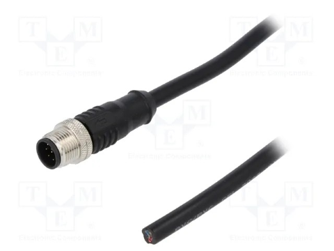

I chose more robust connectors with better IP67 protection for outdoor use. The e-paper display is an optional accessory (it does not have to be connected) if you want to see the measured values at the station's location. Its advantage is that it displays data even when the power is disconnected, and its average power consumption during refreshing is 26.4 mW; outside this period, the current draw is less than 10 nA, so it consumes almost nothing. The disadvantage is the longer refresh time – about 14 seconds, during which the display flickers, which is compensated by its low price. I set the interval to 15 minutes, but this value can be changed as desired. I connected the I2C sensor BM688 to connector XS3, which provides data on temperature, atmospheric pressure,humidity, and air quality with high precision . Connector XS4 is a reserve for planned connection of additional sensors, for example UV radiation, soil moisture, or something else. Radiation measurement is provided by circuits concentrated on the PCB; the connection diagram of these circuits is shown in Fig3.pdf.
Radiation intensity is measured using a Geiger-Müller tube (hereinafter GM). The principle is simple: a glass GM tube is filled with a noble gas, usually neon, argon, …, or a mixture of noble gas and a halogen such as chlorine or bromine. It contains two electrodes to which a high DC voltage of 400 V–600 V is applied. The passage of a particle through the gas triggers an ionizing discharge, which manifests itself as a current pulse on the electrodes. We measure those pulses. The source of the required high voltage applied to the GM tube electrodes is formed by a Cockcroft–Walton (CW) generator, or we can also call it a multiplier. Here we need to pause and chew through a bit of dry theory.
Uoutt = 2 x N x Upeak , wher Upeak is maximum voltage generated by inductor
In order for the high voltage not to drop, it is necessary to appropriately select all parameters of the CW generator, for which the formula for calculating the voltage drop applies:
\[ \Delta V = \frac{ \frac{I}{f C} \cdot N \left( N + 1 \right) \left( 2N + 1 \right) }{12} \]
whre f is input frequency , N is the number of stages, C is the capacitance of the capacitor, and I is the load current.
In the calculation, I assumed that a typical GM tube (e.g., SBM-20) has an operating current of up to 20 µA. An operating frequency between 5 kHz and 10 kHz is recommended; I chose 7 kHz, which the ESP32 can handle well, and the switching transistor will have its operating point far from the cutoff frequency fT. This means that for each single cycle, the required energy is:
\[ E_{cyclus} = \frac{P_{outt}}{f} = 1.43 \times 10^{-6} \, \text{J} \]
whereas the energy in the coil is:
\[ E = \frac{1}{2} L I_{\text{peak}}^2, \quad \text{where} \quad I_{\text{peak}} = \frac{V_{\text{in}} \times t_{\text{on}}}{L}, \quad \text{so} \quad E = \frac{1}{2} L \left( \frac{V_{\text{in}} \times t_{\text{on}}}{L} \right)^2 = \frac{(V_{\text{in}} \times t_{\text{on}})^2}{2L} \]
From these relationships, it is clear that the output high voltage can be conveniently controlled by changing the duty cycle, and for our values HV = 500 V, I = 20 µA, the required power is 10 mW, with coil energy E = 1.43 µJ, the duty cycle will be 23.6% (under ideal conditions).
\[ D = \frac{t_{\text{on}}}{T}, \quad \text{a} \quad t_{\text{on}} = 33{,}8 \, \mu\text{s}, \quad \text{duty is } 23.6\% \]
From these relationships, it can be calculated that at a 50% duty cycle, the output power will be 44.7 mW, and at a 90% duty cycle, the power will be 145 mW. These are theoretical values, but they provide a guarantee that under higher radiation, the source will be able to deliver the necessary power so that the high voltage on the GM tube does not drop and the tube does not lose its ability to ionize the gas and thus generate pulses when an ionizing particle passes through.
From the above theory, it follows that a 3‑stage CW generator is sufficient for the required voltage range of 300 V – 600 V (taking all losses into account). Each stage consists of a pair of diodes and capacitors. During the negative and positive half‑waves of the input AC voltage, the capacitors are gradually charged, and the resulting output voltage is thus a multiple of the input voltage. The input AC voltage for the CW generator is generated by the ESP32 microcontroller on GPIO7 with a frequency of 7 kHz and a variable duty cycle. This allows the output high voltage to be adjusted over a wide range. These variable‑duty‑cycle pulses drive transistor Q2 through resistor R12. When transistor Q2 is open, current flows through the coil, creating a magnetic field in the coil core; when the transistor closes, the energy of this magnetic field induces a voltage across the coil terminals. These voltage spikes have an amplitude of up to 200 V, which is then utilized by the subsequent CW generator formed by diodes D1, D2, D3 and capacitors C4, C5 and C10. Theoretically, up to 1200 V can be achieved with a three‑stage CW generator, which is optimistic and does not take into account the real parameters of the components (transition resistances, parasitic capacitances, switching slope of the transistor, etc.).
I verified the theoretical calculations of the CW generator by practical measurement of the values:
| Desired value [V] | Output voltage [V] | Duty cycle [%] | Deviation [V] | Deviation [%] |
| 100,00 | 228,41 | 9,97 | -128,41 | -128,41 % |
| 125,00 | 228,19 | 9,97 | -103,19 | -82,55 % |
| 150,00 | 228,43 | 9,97 | -78,43 | -52,28 % |
| 175,00 | 228,05 | 9,97 | -53,05 | -30,31 % |
| 200,00 | 228,11 | 9,97 | -28,11 | -14,05 % |
| 225,00 | 228,18 | 9,97 | -3,18 | -1,41 % |
| 250,00 | 245,17 | 11,14 | 4,83 | 1,93 % |
| 275,00 | 268,75 | 12,90 | 6,26 | 2,27 % |
| 300,00 | 296,34 | 14,86 | 3,66 | 1,22 % |
| 325,00 | 320,78 | 16,42 | 4,22 | 1,30 % |
| 350,00 | 347,01 | 18,38 | 2,99 | 0,85 % |
| 375,00 | 374,65 | 20,43 | 0,35 | 0,09 % |
| 400,00 | 394,64 | 21,99 | 5,37 | 1,34 % |
| 425,00 | 421,74 | 24,15 | 3,26 | 0,77 % |
| 450,00 | 447,34 | 26,20 | 2,66 | 0,59 % |
| 475,00 | 470,50 | 28,15 | 4,50 | 0,95 % |
| 500,00 | 495,73 | 30,40 | 4,27 | 0,85 % |
| 525,00 | 522,33 | 32,85 | 2,67 | 0,51 % |
| 550,00 | 545,59 | 35,19 | 4,41 | 0,80 % |
| 575,00 | 571,65 | 38,22 | 3,35 | 0,58 % |
| 600,00 | 596,20 | 40,96 | 3,80 | 0,63 % |
| 625,00 | 620,15 | 44,48 | 4,85 | 0,78 % |
| 650,00 | 644,96 | 48,29 | 5,04 | 0,78 % |
| 675,00 | 670,13 | 52,79 | 4,87 | 0,72 % |
| 700,00 | 696,30 | 58,75 | 3,71 | 0,53 % |
| 725,00 | 723,70 | 65,69 | 1,30 | 0,18 % |
| 750,00 | 712,11 | 89,93 | 37,89 | 5,05 % |
| 775,00 | 712,22 | 89,93 | 62,78 | 8,10 % |
| 800,00 | 711,80 | 89,93 | 88,20 | 11,02 % |
I was interested in how the circuit would behave, including the PID controller. The accuracy of the measured results is affected by the DEADBAND value of the PID controller (explained below), which I set to 5 V. The graph in the figure... Shows the relationship between the desired and actual output high voltage values. From the graph it can be seen that the relationship is practically linear in the range of 250 to 700 V. The graph showing the dependence of the width of the CW generator driving pulses (duty cycle) shows
  this figure. It cannot be expected that the CW generator will work well if the duty cycle is less than 10% or greater than 90%, therefore the possible duty cycle values are limited to this range. The theoretical assumption (according to the calculation) stated that we would reach 500 V at a duty cycle of 23.6%. For 500 V, the actual measured duty cycle value is 30.4%, which is a perfect result because transistor Q2 is not an ideal switching element, and given that it is a transistor with a high collector-emitter blocking voltage, it can be expected that the current gain factor h₂₁ₑ will be on the order of tens, which means higher losses during both the rising and falling edges due to the limited base current that the GPIO output of the ESP32 can provide. The duty cycle value is only informative for assessing agreement with theory. How the transistor's switching characteristics affect agreement with theory can be illustrated with this example. When I replaced resistor R12 (value 2.7 kΩ) in the base of transistor Q2 with a 10 kΩ resistor, the duty cycle changed from 30% to 43% at 500 V output. I mention this only to illustrate how important the switching characteristics of transistor Q2 are for the proper operation of the CW generator. In this circuit, it is not critical because the PID controller takes care of setting the correct output voltage. It would be critical in an open-loop control application. The following graph shows the percentage deviation between the desired and actual values:
From the graph it can be seen that the accuracy of setting the output voltage corresponds to expectations.
The high voltage (HV) thus created is applied through resistor R6 to one electrode of the GM tube, and through a voltage divider (R1+R2+R3+R4+R5)/R16 this HV is reduced to one thousandth and, via filter C9, R11, C11, is fed to GPIO6, which is configured as an ADC input. So, if the HV is 500 V, the ADC input sees 0.5 V. A software PID controller maintains the required HV on the GM tube electrode, which can be set via the configuration web page, and its set value depends on the GM tube used. The PCB is designed to allow different types of GM tubes to be used. Diodes D6 and D7 provide protection for the ADC, whose input voltage should be in the range 0 V – 1 V. The total voltage drop across these two diodes (when conducting) is about 1.1 V, which protects the ESP32 from destruction. Applying 3 V or 5 V to this input in ADC mode would reliably destroy the ESP32 (I haven't tried it, I trust the manufacturer). Since GM tubes have a relatively wide HV range in which they operate reliably, I did not worry about the divider accuracy; I used 1% resistors, so the measurement accuracy (if we neglect ADC non‑linearity and noise, it could be 2%) is certainly better than 5%. GPIO8 and GPIO9 of the microcontroller are used for the I2C bus to communicate with other devices. Diodes D9–D12 protect the bus from induced overvoltage. Pulses from the GM tube caused by ionising radiation are conditioned by divider R7, R15, C3 and are fed to GPIO1, where they are counted by the software. From these, the radiation value in Sieverts per hour is calculated. Via voltage divider R7/R14, the 5 V supply voltage is fed to GPIO2, which is configured as a second ADC input. Diodes D5 and D7 provide protection as already described, and resistor R9 with capacitor C8 ensure filtering and stability during voltage measurement. Through output GPIO10 and transistor Q1, a piezo buzzer BUZZER1 is driven for acoustic alarm when threshold values are exceeded. Its use is not necessary and is not critical for the proper function of the LK‑29 weather station. Inductor L1 and the other capacitors serve filtering purposes and are intended to prevent interference from penetrating the measurement sections of the circuits.
All components are placed on a single double‑sided PCB measuring 140 × 80 mm (120 × 80 mm). The bottom side of the PCB layout, the top side, the assembly drawing and its 3D view are shown in the following figures.


The space for the GM tube is designed so that any GM tube smaller than 120 mm can be used.
I decided to design the printed circuit board using THT (Through‑Hole Technology) so that it can be easily built in amateur conditions even by less experienced radio amateurs. The shape of the PCB corresponds to the dimensions of the Kradex ZP15010060UJPH‑PC enclosure

into which I built it. The protrusions on the left and right sides of the PCB can be broken off or cut off; then the PCB has a standard size of 120 × 80 mm. The enclosure has IP65 protection, which is suitable even for adverse weather conditions that may prevail outdoors. A suitable housing for the sensor was 3D‑printed, including its holder. An image of the assembly model, including the supply cable and PG7 cable gland, is shown in the following figure.
The circular housing has oval openings around its circumference to allow air to flow well to the sensor. Inside, I placed a stainless steel mesh from a plumbing Y‑strainer with 400 µm openings to prevent insects and spiders from entering.
It is clear that a suitable location must be chosen without direct sunlight on the sensor so that the air temperature data is reliable.
Software
All required functions are controlled by software. The program ensures the reading and conversion of values from the sensors, their display on the local ePaper display, or remotely in a web browser via the HTTP protocol. It also manages the Wi-Fi network connection. The program has a modular architecture; here is a list of the most important modules:
|
The most important program modules |
|
|
File |
Description |
|
main.py |
main control loop, module initialization |
|
reg.py |
regulation HV, ADC, GM pulses, CPM |
|
i2c.py |
communication with BME688 / SHT30 |
|
openweather.py |
reading forecst from OpenWeatherMap |
|
geoip.py |
IP geolocation |
|
display.py |
ePaper display |
|
influx.py |
write records to InfluxDB |
|
wifi_manager.py |
Wi-Fi connection management |
|
http_server.py |
HTTP server |
|
http_api.py |
API handlers |
|
config.py |
configuration variables |
|
http_cfg.py |
web interface variable |
|
html/dashboard.html |
The Dashboard is the main user screen accessible at http://<ip>/ or http://<ip>/dashboard. It is optimized for both mobile devices and computers (responsive design). |
|
html/dashboard.css |
contains display styles for different formats and display orientations. |
|
html/http_server.json |
defines the structure of the web interface. |
I also considered using the HTTPS protocol, but the security benefit is minimal. The device runs on a local network, and SSL protects against eavesdropping on data in transit between the browser and the server, but on a home Wi‑Fi this risk is practically zero. The real threat (if any) is unauthorised access, and SSL does not solve that (anyone on the network can connect via HTTPS just as easily as via HTTP). That is addressed by using a password for the configuration pages. Since the ESP32 does not have a domain name or a CA‑signed certificate, I would have to use a self‑signed certificate. Every browser will show a warning: "This connection is not secure" and you would have to click "Proceed despite the risk". On a mobile device in kiosk mode (Fully Kiosk), this can be a problem — some WebViews refuse it completely. The dashboard polls every 15 s and my dashboard.html calls /api/data every 15 s. Each request would require a full TLS handshake (the ESP32 does not maintain keep‑alive with TLS), which on an ESP32‑S3 takes 1–2 seconds. This would slow down the dashboard response and load the processor. Also RAM usage during the TLS handshake. With TLS connections on the ESP32, ENOMEM errors (not enough memory) appear, and the handshake itself consumes 30–50 KB of RAM per connection. If the dashboard opens several requests simultaneously (data + CSS + JS), the program may crash.
After a restart, the boot.py program runs, which is created when MicroPython is flashed into the memory. It does not need any modification, because after loading boot.py, MicroPython automatically runs main.py if it exists. Our main.py loads the configuration from config.py, then reg.py runs, which initialises PWM, ADC, GM pins, the PID controller and the CPM timer (for counting pulses from the GM tube). The I2C bus, OpenWeatherMap, GeoIP (optional) are initialised, and it tries to connect to Wi‑Fi (the Wi‑Fi configuration is stored in the file wifi_config.json). If connection fails, it starts AP mode "LK-29 Setup", where the Wi‑Fi module of the ESP32 switches to AP mode, and after connecting to the AP, the configuration screen is available at http://192.168.4.1, which calls the wifi_manager.py program allowing scanning of nearby available networks and connecting to them, or manually setting network parameters. After pressing the "Connect" button, the microprocessor tries to connect to the Wi‑Fi network, and if successful, it switches to client mode and restarts. After restart and successful Wi‑Fi connection, it continues by starting the HTTP server and initialising the ePaper display. Then the program stays in the main loop and services HTTP, I2C reading, OpenWeatherMap updates, InfluxDB writes, ePaper display (if present). In the main loop, the program "loafs around" because all important activities are managed via interrupts, including timing loops. The high voltage is set and stabilised by a PID controller, which runs in a timer interrupt (default 100 ms), reads the ADC value via the divider feedback, compares the read value with the TARGET_VOLTAGE variable, calculates the PID output and adjusts the PWM duty cycle. If the error (difference between desired and actual voltage) is within the deadband (allowed deviation from the desired voltage), the integral component is reset.
 Counting pulses from the GM tube is also performed using an interrupt. A current pulse from the GM tube triggers an interrupt on the GPIO1 input, which increments a variable containing the pulse count. An interrupt from a timer, which occurs every 60 seconds, calculates the difference between the old and new pulse count, thus obtaining the current CPM (counts per minute) value, which represents the number of ionising particles that have excited the gas in the tube. From this data, the radiation value in microsieverts per hour (µSv/h) is also calculated. This calculation is governed by its own timer to improve accuracy, especially for smaller tubes, such as the Xeram 3G8B, which I also used. The relationship between CPM and intensity expressed in µSv/h is defined by the manufacturer, and its value is stored in the appropriate variable CPM_PER_USV in config.py. The radiation dose is calculated as follows:
\[ \text{dose} \left( \frac{\mu\text{Sv}}{\text{h}} \right) = \frac{\text{CPM}}{\text{CPM\_PER\_USV}} \]
Temperature, humidity, … values are read from I2C sensors. Automatic detection of the presence of a sensor is performed during the first scan (10 s after startup). Then it is read at intervals of I2C_INTERVAL seconds. The BME688 provides temperature, humidity, pressure and IAQ (air quality) value. At the set OWM_INTERVAL, the current weather and 5‑day forecast are retrieved (default 1800 s = 30 min). If no I2C sensor is available, temperature and humidity are taken from OWM (OpenWeatherMap, or Open‑meteo). For further processing of the measured data, it is possible to store the data in a database. If INFLUX_ENABLED = True, the system writes the measured values to an InfluxDB database at regular intervals INFLUX_INTERVAL (seconds). The following are written: temperature, humidity, pressure, radiation dose, CPM, battery voltage, etc. The value of the variable DISPLAY = True indicates the presence of an ePaper display; the system updates the values on the ePaper display at the interval REFRESH_DISP (number of seconds). It displays the current values from the sensors, the calculated radiation dose and the status.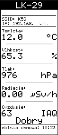
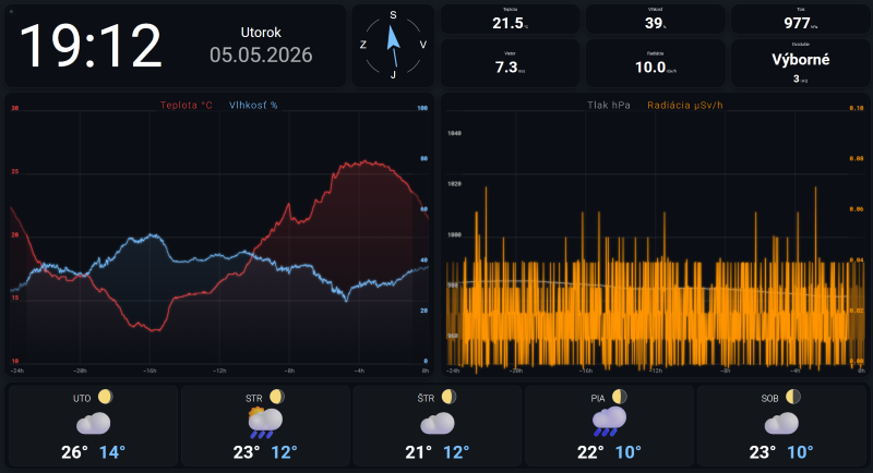 An important part is the web interface via the HTTP server. The main screen is available at http://<IP_address>/ or http://<IP_address>/dashboard.html. The appearance can be controlled via CSS files. Loading data into the page, automatic refresh and displaying graphs are handled by JavaScripts in the HTML code. The interface is available in two language versions, and adding another language is done by creating a JSON file with the appropriate translation. For example, for Czech it is enough to translate the contents of
 lang_en.json into Czech and name it lang_cz.json. Then set the language to "cz" in the configuration interface. The file manifest.json is also important, referenced by the so‑called PWA manifest (it tells the browser and operating system how your application should look and behave when the user installs it on the device's desktop, start menu, or phone home screen). Every HTML file on the HTTP server references it in its code, thus ensuring correct display on different devices (portrait/landscape mode on a mobile phone or tablet, full‑screen mode, etc.). Sizes and positions change dynamically according to the displayed window (responsive design). At http://<IP_address>/api/data, most variables are available for further processing. This is advantageous for possible integration and transferring values to other systems. An example is displaying data in Home Assistant (smart home software) without the need for additional integration using the built‑in RESTful system integration. The dashboard stores the last 1440 measured points (24 hours) in the ESP32's RAM. With each new point (every minute), the array is updated and the graphs are redrawn. This means that if data is cleared in the browser, or the browser is launched on another device, the graphs for the last 24 hours are rendered. This data is available at http://<IP_address>/api/history. The time is synchronised with an NTP server at startup and then at intervals of SYNC_INTERVAL_DEV hours. The time zone offset and DST are set in config.py. The dashboard automatically switches to full‑screen mode after the first click (due to PWA). If the user exits full‑screen, the device tries to reactivate it on the next interaction.
Full‑screen mode does not work on some mobiles and tablets in the Chrome browser. My code in dashboard.html tries to force full‑screen via the JavaScript API on the first click/touch. Chrome distinguishes between different display modes and requestFullscreen() has strict rules on tablets. Moreover, on some tablets Chrome respects the system navigation bar settings and refuses full‑screen. If the tablet is to serve as a permanent display, the Fully Kiosk Browser application is the most reliable solution. It provides native full‑screen without navigation elements, auto‑start after boot, and screen‑on management. My dashboard works well with it on both phones and tablets.
Dashboard charts can be customized using a drag-and-drop function: simply place your finger or mouse cursor on the tile representing the value you wish to view and drag it into the chart area.
A quick tap or click on a tile displaying a measured value will show the maximum and minimum values recorded over the last 24 hours, which also corresponds to the chart's x-axis range, for a duration of seven seconds.
Most functions of the weather station are displayable via the web interface. This way, it is also possible to view the content rendered on the ePaper display or to monitor what is being printed to the ESP32 console, for example logs.
 . A description of other options can be found in the user manual, and all necessary software can be downloaded from https://www.dedeideas.eu in the download section.
Control panel
The configuration of the LK‑29 weather station parameters is concentrated in the config.py module, the so‑called 'Control panel'. All important variables are also available via http://<IP_address>/config.. 


 Access requires username and password authorization. The username is fixed to "admin" and the password is empty by default. The control panel is divided into six sections.
The first two sections are "Live Measurements" and "Wi‑Fi Status". In the upper left corner of the screen there is a ☀ or ☾ icon, allowing switching between dark and light style (day/night). The "Live Measurements" section shows the current measured important values. I think they do not need to be described; their meaning is clear from the previous description of the weather station. The second section, "Wi‑Fi Status", displays the current network connection parameters. All data is read‑only except for the gear icon ⚙ in the "Status" row. Clicking this button invokes the network connection settings screen (Wi‑Fi Manager), which allows scanning of surrounding networks and connecting to them.
The second figure shows the next two sections of the control panel. The "I2C Bus" section displays data about devices on the I2C bus. Pressing the gear icon ⚙ in the status row triggers a rescan of the I2C bus. Found devices, their addresses and types are printed in the row below. In this version, the program can handle SHT3x and BME68x I2C devices. The "Read Only Configuration" section displays important system values; they cannot be edited, only read.
The next section, "OpenMeteo/OpenWeatherMap", displays information about reading from the weather forecast source. Clicking the gear icon ⚙ forces a reload of new data from the weather forecast source. The largest section is the "Editable configuration" section, which contains several groups (Firmware, OpenMeteo/OpenWeatherMap, Bat divider, …).
The first group in the "Editable configuration" section is for firmware upgrade over Wi‑Fi. After clicking the "Upgrade" button, the page http://<IP_address>/ota opens, where you can enter the name of a ZIP file containing the program package. All files in the ESP32 flash memory will be deleted, including subdirectories, and the contents of the ZIP file will be unpacked and copied into flash memory. The ZIP file can be with normal compression or without compression. The progress of unpacking and copying files is shown in the status bar and in the upgrade frame. After the files are unpacked, the ESP32 restarts automatically. In the "OpenMeteo / OpenWeatherMap" group, you can choose the weather forecast source. OpenMeteo requires no settings other than location (Latitude, Longitude), which you can obtain from Google Maps. OpenWeatherMap requires an API key (OWM), which you can obtain for free after registering on the OpenWeatherMap website.
 The next group, "BAT divider", contains only one item – "VBAT divider ratio", which is a correction coefficient for measuring battery or supply voltage. The supply voltage is fed to the ADC input via a voltage divider R8/R14. I used standard resistors which do not have high precision nor exact division ratios. I connected a voltmeter to the supply terminals and set the "VBAT divider ratio" coefficient so that the voltage on the voltmeter and the "Battery Voltage" in the "Live Measurements" section showed the same value.
The next group, "HV regulator", concerns the high‑voltage PID controller. In the "Target voltage" item, you set the desired high voltage for the GM tube according to the type you have used, to the value specified by the manufacturer. Usually, the manufacturer gives the minimum high voltage – the "threshold voltage" – at which discharge occurs in the tube. Typically this value is between 300 V and 400 V and marks the beginning of the so‑called "Geiger plateau", which is the high‑voltage region above the threshold voltage where the tube reliably detects ionising radiation particles, and is usually more than 200 V wide. So I recommend setting this value to threshold voltage + 50 V or +100 V. I used the Xeram 3GB8 GM tube, for which the manufacturer states that the threshold voltage is 445 V. When I set it to 450 V, the tube reliably detected radioactive particles from the natural background. I set it to 500 V so that any drop in high voltage would not distort the measurement. The other parameters relate to setting the PID controller and I do not recommend changing them unless you know what you are doing. The next group, "Buzzer", has only one item – a checkbox "Acoustic signalling" to enable/disable acoustic indication of detected particles. The "Radiation" group, in the "CPM per 1 µSv/h" item, determines the number of detected particles per minute (CPM) for calculating 1 µSv/h. This data is defined by the GM tube manufacturer – look for it in its documentation. The "Alarm threshold" item sets the radiation value at which the acoustic alarm signals elevated radiation. The value in the "CPM calc period" row represents the number of milliseconds indicating how often the CPM value is recalculated into the radiation dose in µSv/h.
In the next group, "I2C Sensors", you set the time intervals for reading values from I2C sensors and refreshing the e‑paper display. I remind you that the time needed to fully redraw the display is 14 seconds, during which the display flickers and is not easy to read, so too low a refresh interval would be disturbing. The "Time" group allows setting time and language interface data.
 The "InfluxDB" group brings together the settings for writing measured values to the database. Two lines in this group are worth attention: "Buffered records" and "DB buffer capacity". The former tells how many records are ready in the ESP32 microcontroller's RAM to be written to the database if it is unavailable; this value can be overwritten to a smaller number or even zeroed, which permanently loses the unsaved records from the ESP32's RAM. The second value tells how many records the ESP32 will hold in memory until database access is restored, so that old records can be stored. You can enter any large value, but it is checked against RAM requirements and the maximum value that does not consume more than 90% of free RAM is calculated. Memory is allocated only when a new record is created, so this value does not affect immediate RAM usage. With this hardware configuration, the maximum value is around 8000 records, which at minute‑interval data collection represents about one week. The data is in a circular buffer, meaning that once the maximum number of records in the buffer is reached, the oldest is deleted when a new one is added. A power loss means loss of the buffer contents, since I decided not to "bother" with saving records to flash. The "Debug level" group allows you to select which program modules should produce detailed log outputs, for example the high‑voltage regulator module. I do not recommend leaving logs enabled, because the outputs are directed to the ESP32 console. The reason is that most serial outputs are blocking. This means that when sending each character, the processor waits for it to be physically transmitted, and during that time it cannot perform any other useful work. And although the ESP32‑S3 is a fast processor, the serial line speed (typically 115200 baud, which is ~11 kB per second) is extremely slow in comparison, so such overhead dominates the total program runtime and significantly slows down its response. Clicking the small square button ✓ at the end of the line causes the value to be set immediately, which also takes effect right away, but it is not saved to the configuration file in flash memory, with the result that a change made this way is valid only until the next restart, whereupon initialisation sets the values according to the settings stored in the ESP32's flash memory. Acceptance of the new value is signalled by the button's background colour changing for two seconds ✓ . The "Save config" button in the last group is used to permanently save the changed values. The "Download config" button allows downloading the configuration file to the local computer. The other two buttons have an obvious meaning. "Restart" is used to restart the ESP32, and "Change PWD" is used to change the password for accessing the configuration panel. If you lose the password, the only option is to connect to the ESP32 via the serial port and in config.py set the variable AUTH_PASSWORD = "" as empty or to the desired value. Changing some parameters requires a restart; this is indicated by the background of the "Restart" button turning red, meaning that a restart of the ESP32 is required as soon as possible.